Chapter 4 Analysis with synthetic data

In this section we describe how we can use a copy of the synthetic data to help users write DataSHIELD analysis code. Again we will make use of an existing data set.

Recall that the objective here is to use a synthetic copy of already harmonised real data that is then made available to the analyst on the client side. This synthetic data set can be loaded into DSLite, a special client side implementation of server side DataSHIELD used for development purposes. DSLite is will only take standard DataSHIELD functions as input, but the user can have full access to the data through a special interface. This is acceptable in this situation as the data are synthetic and designed to be non-disclosive. Therefore the user has the chance to write DataSHIELD code but see the complete results of each step. This makes it easier to develop the code.

The steps are summarised as:

User requests synthetic copy of real data
Synthetic data generated & available on client side
Synthetic data placed in DSLite environment that simulates server side DataSHIELD environment
Develop DataSHIELD code against synthetic data in DSLite (with full access to synthetic data)
When DataSHIELD code is complete, run code against real data on server side

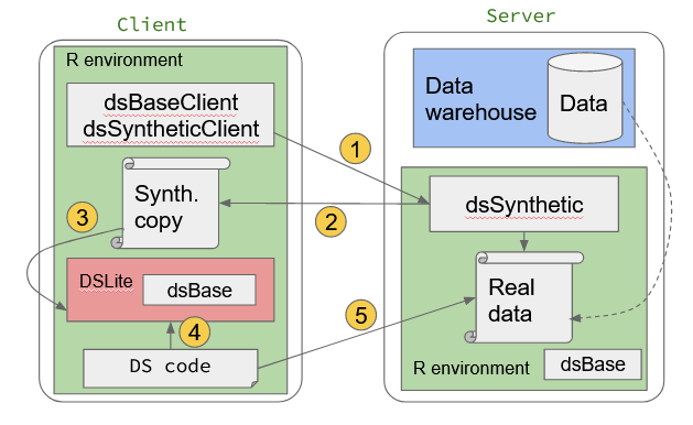
Figure 4.1: Prototyping DataSHIELD analysis using synthetic data on DSLite

4.1 Getting set up

Let us assume that the DASIM1 dataset has previously been harmonised and is held on a server. As normal with DataSHIELD, we do not have complete access to the full data set but want to do some analysis on it. Using the method described above, the first thing to do is generate a synthetic version of the data that we can fully access. To do this we will use the same steps that were shown in 3

We build our log in object

builder <- DSI::newDSLoginBuilder()
builder$append(server="server1", url="https://opal-sandbox.mrc-epid.cam.ac.uk",
               user="dsuser", password="P@ssw0rd", 
               table = "DASIM.DASIM1")
logindata <- builder$build()

Then perform the log in to the server:

library(DSOpal)
if(exists("connections")){
  datashield.logout(conns = connections)
}
connections <- datashield.login(logins=logindata, assign = TRUE)

4.2 Create synthetic dataset

The DASIM1 dataset is relatively small (i.e. around 10 columns). This is probably also true of many harmonised data sets. Therefore we can just create a synthetic version of it in its entirety without specifying a subset of columns:

library(dsSyntheticClient)
synth_data = ds.syn(data = "D", method = "cart", m = 1, seed = 123)
# N.B. you may need to replace `server1` if you have named your connection differently
DASIM = synth_data$server1$Data$syn

4.3 Start DSLite local instance

Here we start our DSLite instance, and load the DASIM data. Recall that this simulates the server side environment on your client, but with the ability to access all the data. Therefore it is ideal for our requirement to build a code pipeline while being able to see the data: this helps with the debugging and logic checking process.

library(DSLite)
library(dsBaseClient)
dslite.server <- newDSLiteServer(tables=list(DASIM=DASIM))
dslite.server$config(defaultDSConfiguration(include=c("dsBase", "dsSynthetic")))

builder <- DSI::newDSLoginBuilder()
builder$append(server="server1", url="dslite.server", table = "DASIM", driver = "DSLiteDriver")
logindata <- builder$build()

if(exists("connections")){
  datashield.logout(conns = connections)
}
connections <- datashield.login(logins=logindata, assign = TRUE)

We can now check for ourselves that our DASIM data is in the DSLite server:

ds.summary('D')

## $server1
## $server1$class
## [1] "data.frame"
## 
## $server1$`number of rows`
## [1] 10000
## 
## $server1$`number of columns`
## [1] 10
## 
## $server1$`variables held`
##  [1] "LAB_TSC"            "LAB_TRIG"           "LAB_HDL"           
##  [4] "LAB_GLUC_FASTING"   "PM_BMI_CONTINUOUS"  "DIS_CVA"           
##  [7] "DIS_DIAB"           "DIS_AMI"            "GENDER"            
## [10] "PM_BMI_CATEGORICAL"

4.4 Write some analysis code

Now suppose we want to subset the DASIM data into men and women. We can use the ds.subset function:

ds.subset(x="D", subset = "women", logicalOperator = "==", threshold = 1)

With DSLite we have the chance to look at actually what happened in detail:

# N.B. you may need to replace `server1` if you have named your connection differently
women = getDSLiteData(conns = connections, symbol = "women")$server1
head(women)

##        LAB_TSC  LAB_TRIG   LAB_HDL LAB_GLUC_FASTING PM_BMI_CONTINUOUS DIS_CVA
## 1     5.716675 1.2131437 1.2263569         4.746905          28.30447       0
## 10    5.635550 1.0352904 0.9980688         4.724115          26.40500       0
## 100   4.304612 0.2782473 1.7977266         3.922677          28.83399       0
## 1000  6.250217 0.8718639 1.8747723         3.457615          23.08530       0
## 10000 8.621496 4.3548597 1.1010694         4.637112          27.85634       0
## 1001  5.026787 2.2295412 1.1088745         3.802152          21.22769       0
##       DIS_DIAB DIS_AMI GENDER PM_BMI_CATEGORICAL
## 1            0       0      0                  2
## 10           0       0      1                  2
## 100          0       0      1                  2
## 1000         0       0      1                  1
## 10000        0       0      0                  2
## 1001         0       0      0                  1

This doesn’t look quite right. There are still rows with GENDER == 0. There is an error in our code (we didn’t specify GENDER as part of the logicalOperator parameter) but didn’t get a warning. Let’s make a correction and try again:

ds.subset(x="D", subset = "women", logicalOperator = "GENDER==", threshold = 1)
# get the data again
# N.B. you may need to replace `server1` if you have named your connection differently
women = getDSLiteData(conns = connections, symbol = "women")$server1
head(women)

##       LAB_TSC   LAB_TRIG   LAB_HDL LAB_GLUC_FASTING PM_BMI_CONTINUOUS DIS_CVA
## 10   5.635550  1.0352904 0.9980688         4.724115          26.40500       0
## 100  4.304612  0.2782473 1.7977266         3.922677          28.83399       0
## 1000 6.250217  0.8718639 1.8747723         3.457615          23.08530       0
## 1002 5.743905  2.6050324 1.0818273         4.285118          30.99263       0
## 1004 4.054283 -0.8651860 2.3976915         4.419434          23.00676       0
## 1005 4.565802  1.8247904 1.4323840         5.322401          36.89399       0
##      DIS_DIAB DIS_AMI GENDER PM_BMI_CATEGORICAL
## 10          0       0      1                  2
## 100         0       0      1                  2
## 1000        0       0      1                  1
## 1002        0       0      1                  3
## 1004        0       0      1                  1
## 1005        0       0      1                  3

This now looks much better.

4.5 Run corrected code on real data

We can also compare results obtained via DataSHIELD with results on the actual data:

from_server = ds.glm(formula = "DIS_DIAB~PM_BMI_CONTINUOUS+LAB_TSC+LAB_HDL", data = "women", family = "binomial")
from_local = glm(formula = "DIS_DIAB~PM_BMI_CONTINUOUS+LAB_TSC+LAB_HDL", data = women, family = "binomial")

from_server$coefficients

##                     Estimate Std. Error   z-value      p-value low0.95CI.LP
## (Intercept)       -5.9908647 0.95366097 -6.281965 3.343205e-10  -7.86000582
## PM_BMI_CONTINUOUS  0.1428793 0.02249027  6.352938 2.112405e-10   0.09879916
## LAB_TSC           -0.2090230 0.09820091 -2.128524 3.329370e-02  -0.40149320
## LAB_HDL           -0.5191230 0.28273998 -1.836044 6.635116e-02  -1.07328321
##                   high0.95CI.LP        P_OR low0.95CI.P_OR high0.95CI.P_OR
## (Intercept)         -4.12172352 0.002495258   0.0003857228      0.01595776
## PM_BMI_CONTINUOUS    0.18695938 1.153590520   1.1038445800      1.20557831
## LAB_TSC             -0.01655271 0.811376611   0.6693198696      0.98358354
## LAB_HDL              0.03503715 0.595042151   0.3418841935      1.03565818

from_local$coefficients

##       (Intercept) PM_BMI_CONTINUOUS           LAB_TSC           LAB_HDL 
##        -5.9908647         0.1428793        -0.2090230        -0.5191230